
The concept of using an X-ray source coupled with a detector as a microscope was originally detailed by V E Cosslett & W C Nixon in their publication “A point X-ray focus for Shadow microscopy” in 1951. This was later implemented by Professor Jim Cornelis Elliott and David Dover in the early 1980’s in the development of the first laboratory based X-ray micro tomography system. These original works define modern X-ray CT laboratory systems.
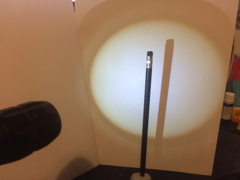
A practical demonstration of this principle can be achieved with a simple light source such as a small torch. Place the torch a small distance (i.e 0.5m) away from a white background and place an object between the torch and the background. As the object is moved towards the torch the shadow increases in size due to the magnification effect, while moving the object towards the wall results in less magnification and a smaller image. At high magnifications a blurring of the objects edges occurs and this will be described later under sections of image quality and focal spot blur.
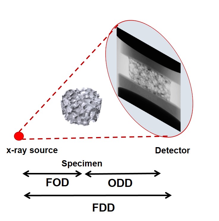
To calculate the magnification and effective pixel size the following factors need to be known:
- Focal spot of the X-ray source to Detector Distance (FDD)
- Focal spot to Object Distance (FOD)
- Pixel pitch of the detector (Pp), this is the physical size of the pixels that make up the detector
The geometric magnification (M) is calculated using the FDD and FOD as shown below:
The effective pixel size (Ps) is the pixel size due to the magnification effect. This is calculated from the pixel pitch of the detector and the geometric magnification as follows:
Ps = Pp / M
For a given magnification the Field of View (FoV) on the detector can be calculated from the effective pixel size and the number of pixels across the horizontal plane (Np) of the detector as follows:
FoV = NpPs
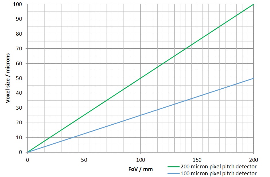
This information can then be used to perform useful calculations to determine the systems capability regarding different sized objects. The most useful graph that can be produced is the FoV vs Effective pixel size as shown opposite. The graph is useful for predicting the achievable resolution for objects of a specific size. In the example the calculation is shown using detectors with a pixel pitch of 100 and 200 microns. The smaller the pixel pitch the better the magnification and smaller the effective pixel size for an equivalent FoV.
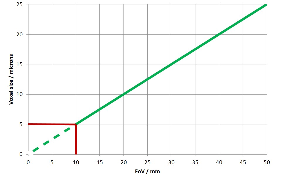
In theory the effective pixel size will continue to decrease until the FoV reaches zero. However there is a practical limit beyond which a decrease in pixel size has no effect upon the spatial resolution. This limit is determined by the focal spot size of the X-ray source. The smaller the X-ray focal spot size the better the spatial resolution. This is explained in the sections detailing X-ray sources and spatial resolution. Generally a good rule of thumb is that decreasing the effective pixel size below the effective spot size does not improve spatial resolution. In the example on the right the focal spot size is shown as a red line at 5 microns, decreasing the pixel size or the FoV (or object size) will not result in a better spatial resolution.